Time-to-event data analysis with the bmstate package

library(bmstate)
#> Attached bmstate 0.2.7. Type ?bmstate to get started.
library(ggplot2)
library(dplyr)
#> 
#> Attaching package: 'dplyr'
#> The following objects are masked from 'package:stats':
#> 
#>     filter, lag
#> The following objects are masked from 'package:base':
#> 
#>     intersect, setdiff, setequal, union
library(tidyr)
library(ggdist)
theme_set(theme_bw())

Data

Data preprocessing

Here we analyse the cav data from the msm package. It is a Cardiac Allograft Vasculopathy (CAV) data set of 622 heart transplant recipients. They are observed either in state 1 (No CAV), state 2 (Mild CAV), state 3 (Severe CAV), or state 4 (Dead).

First we modify the original data like here.

df_full <- as_tibble(msm::cav) |>
  group_by(PTNUM) |>
  mutate(
    min_age = min(age),
    state = cummax(state)
  )
head(df_full)
#> # A tibble: 6 × 11
#> # Groups:   PTNUM [1]
#>    PTNUM   age years  dage   sex pdiag cumrej state firstobs statemax min_age
#>    <int> <dbl> <dbl> <int> <int> <fct>  <int> <int>    <int>    <dbl>   <dbl>
#> 1 100002  52.5  0       21     0 IHD        0     1        1        1    52.5
#> 2 100002  53.5  1.00    21     0 IHD        2     1        0        1    52.5
#> 3 100002  54.5  2.00    21     0 IHD        2     2        0        2    52.5
#> 4 100002  55.6  3.09    21     0 IHD        2     2        0        2    52.5
#> 5 100002  56.5  4       21     0 IHD        3     2        0        2    52.5
#> 6 100002  57.5  5.00    21     0 IHD        3     3        0        3    52.5

This is snapshot data of the state at given time rather than exactly observed transition times. Only the death times are exact. We make an assumption that all state transitions happen exactly at the first time the new state is seen in the data.

We select only needed columns and rename them. In our resulting data frame, we will have columns

time: time since transplant (in years)
age: age of the patient at transplant time
dage: age of the donor
sex: 0 or 1

df_full$PTNUM <- as.character(df_full$PTNUM)
df_snapshots <- df_full |> select(PTNUM, state, years, min_age, dage, sex)
df_snapshots <- df_snapshots |> rename(
  subject_id = PTNUM,
  age = min_age,
  time = years
)
head(df_snapshots)
#> # A tibble: 6 × 6
#> # Groups:   subject_id [1]
#>   subject_id state  time   age  dage   sex
#>   <chr>      <int> <dbl> <dbl> <int> <int>
#> 1 100002         1  0     52.5    21     0
#> 2 100002         1  1.00  52.5    21     0
#> 3 100002         2  2.00  52.5    21     0
#> 4 100002         2  3.09  52.5    21     0
#> 5 100002         2  4     52.5    21     0
#> 6 100002         3  5.00  52.5    21     0

We remove the unnecessary snapshot rows that are not needed after making the simplifying assumption.

df_state_changes <- df_snapshots |>
  arrange(subject_id, time) |>
  group_by(subject_id) |>
  mutate(
    .first = row_number() == 1,
    .last  = row_number() == n(),
    .chg   = state != lag(state) # TRUE at the first row of each new state run
  ) |>
  filter(.first | .last | .chg | is.na(lag(state))) |> # keep first, last, and changes
  select(-.first, -.last, -.chg) |>
  ungroup()

# Every row is a transition but the first
df_state_changes <- df_state_changes |>
  group_by(subject_id) |>
  mutate(is_transition = tidyr::replace_na(state != lag(state), FALSE)) |>
  ungroup()
head(df_state_changes)
#> # A tibble: 6 × 7
#>   subject_id state  time   age  dage   sex is_transition
#>   <chr>      <int> <dbl> <dbl> <int> <int> <lgl>        
#> 1 100002         1  0     52.5    21     0 FALSE        
#> 2 100002         2  2.00  52.5    21     0 TRUE         
#> 3 100002         3  5.00  52.5    21     0 TRUE         
#> 4 100002         4  5.85  52.5    21     0 TRUE         
#> 5 100003         1  0     29.5    17     0 FALSE        
#> 6 100003         3  2.01  29.5    17     0 TRUE

Transition matrix

We use the following transition matrix, which is built into the package.

tm <- transmat_progression()
tm
#>         Healthy Mild Severe Dead
#> Healthy       0    1      1    1
#> Mild          0    0      1    1
#> Severe        0    0      0    1
#> Dead          0    0      0    0

The PathData format

We format the data as PathData.

covs <- c("age", "dage", "sex")
pd <- df_to_pathdata(df_state_changes, tm, covs)
pd
#> PathData object with 622 paths
#>  * States = {Healthy, Mild, Severe, Dead}
#>  * Covariates = {age, dage, sex}

Analysis

Fitting a model

We create a model and set the spline knot locations based on quantiles of the observed transition times.

# MSM
mod <- create_msm(tm,
  hazard_covs = covs,
  n_grid = 10000,
  t_max = 20
)
t_trans <- pd$transition_times()
mod$set_knots(t_max = 20, t_event = t_trans, num_knots = 3)
mod$get_knots()
#> [1]  0.000000  4.980822 20.000000

We fit the model by optimizing.

fit <- fit_stan(mod, data = pd, method = "optimize")
#> Using stan file at /home/runner/work/_temp/Library/bmstate/stan/msm.stan
#> Initial log joint probability = -362803 
#>     Iter      log prob        ||dx||      ||grad||       alpha      alpha0  # evals  Notes  
#> Error evaluating model log probability: Non-finite gradient. 
#> Error evaluating model log probability: Non-finite gradient. 
#> Error evaluating model log probability: Non-finite gradient. 
#> Error evaluating model log probability: Non-finite gradient. 
#>       99      -1859.49     0.0281839       13.4581           1           1      121    
#>     Iter      log prob        ||dx||      ||grad||       alpha      alpha0  # evals  Notes  
#>      199      -1858.05     0.0152368       1.88641           1           1      227    
#>     Iter      log prob        ||dx||      ||grad||       alpha      alpha0  # evals  Notes  
#>      299      -1857.87    0.00716934       2.13723           1           1      338    
#>     Iter      log prob        ||dx||      ||grad||       alpha      alpha0  # evals  Notes  
#>      399      -1857.79    0.00653108       1.98944      0.1595           1      449    
#>     Iter      log prob        ||dx||      ||grad||       alpha      alpha0  # evals  Notes  
#>      499      -1857.74    0.00123761      0.191422           1           1      556    
#>     Iter      log prob        ||dx||      ||grad||       alpha      alpha0  # evals  Notes  
#>      599      -1857.72     0.0095713      0.502378           1           1      663    
#>     Iter      log prob        ||dx||      ||grad||       alpha      alpha0  # evals  Notes  
#>      699      -1857.71    0.00255015      0.596568           1           1      772    
#>     Iter      log prob        ||dx||      ||grad||       alpha      alpha0  # evals  Notes  
#>      799      -1857.69   0.000664024      0.230892           1           1      880    
#>     Iter      log prob        ||dx||      ||grad||       alpha      alpha0  # evals  Notes  
#>      841      -1857.69   0.000797173     0.0860521           1           1      924    
#> Optimization terminated normally:  
#>   Convergence detected: relative gradient magnitude is below tolerance 
#> Finished in  3.4 seconds.

Inferred baseline hazards

plt <- fit$plot_h0()
plt

Inferred covariate effects

fit$covariate_effects()
#>   covariate         beta target_state_idx target_state
#> 1       age -0.0089 ± NA                2         Mild
#> 2       age -0.0559 ± NA                3       Severe
#> 3       age  0.3135 ± NA                4         Dead
#> 4      dage  0.3429 ± NA                2         Mild
#> 5      dage  0.0458 ± NA                3       Severe
#> 6      dage  0.1009 ± NA                4         Dead
#> 7       sex -0.1583 ± NA                2         Mild
#> 8       sex -0.0761 ± NA                3       Severe
#> 9       sex  0.1411 ± NA                4         Dead

State occupancy probabilities

For each subject, we compute the probability that they are in a given state at time $t$ .

p_state_df <- function(fit, oos, data = NULL) {
  df <- p_state_occupancy(fit, data = data, oos = oos)
  if (is.null(data)) {
    data <- fit$data
  }
  df <- df |> left_join(data$paths$subject_df, by = "subject_id")
  df$State <- paste0(df$state_idx, ": ", df$state)
  df$sex <- as.factor(df$sex)
  df
}
df <- p_state_df(fit, oos = FALSE)
#> Recompiling Stan model
#> Using stan file at /home/runner/work/_temp/Library/bmstate/stan/msm.stan
#> ar: creating stan/lib/stan_math/lib/sundials_6.1.1/lib/libsundials_nvecserial.a
#> ar: creating stan/lib/stan_math/lib/sundials_6.1.1/lib/libsundials_cvodes.a
#> ar: creating stan/lib/stan_math/lib/sundials_6.1.1/lib/libsundials_idas.a
#> ar: creating stan/lib/stan_math/lib/sundials_6.1.1/lib/libsundials_kinsol.a
#> /home/runner/.cmdstan/cmdstan-2.37.0/stan/lib/stan_math/lib/tbb_2020.3/build/Makefile.tbb:28: CONFIG: cfg=release arch=intel64 compiler=gcc target=linux runtime=cc13.3.0_libc2.39_kernel6.11.0
#> In file included from ../tbb_2020.3/src/tbb/concurrent_hash_map.cpp:17:
#> ../tbb_2020.3/include/tbb/concurrent_hash_map.h:347:23: warning: ‘template<class _Category, class _Tp, class _Distance, class _Pointer, class _Reference> struct std::iterator’ is deprecated [-Wdeprecated-declarations]
#>   347 |         : public std::iterator<std::forward_iterator_tag,Value>
#>       |                       ^~~~~~~~
#> In file included from /usr/include/c++/13/bits/stl_construct.h:61,
#>                  from /usr/include/c++/13/bits/stl_tempbuf.h:61,
#>                  from /usr/include/c++/13/memory:66,
#>                  from ../tbb_2020.3/include/tbb/tbb_stddef.h:452,
#>                  from ../tbb_2020.3/include/tbb/concurrent_hash_map.h:23:
#> /usr/include/c++/13/bits/stl_iterator_base_types.h:127:34: note: declared here
#>   127 |     struct _GLIBCXX17_DEPRECATED iterator
#>       |                                  ^~~~~~~~
#> cc1plus: note: unrecognized command-line option ‘-Wno-unknown-warning-option’ may have been intended to silence earlier diagnostics
#> In file included from ../tbb_2020.3/src/tbb/concurrent_queue.cpp:22:
#> ../tbb_2020.3/include/tbb/internal/_concurrent_queue_impl.h:749:21: warning: ‘template<class _Category, class _Tp, class _Distance, class _Pointer, class _Reference> struct std::iterator’ is deprecated [-Wdeprecated-declarations]
#>   749 |         public std::iterator<std::forward_iterator_tag,Value> {
#>       |                     ^~~~~~~~
#> In file included from /usr/include/c++/13/bits/stl_construct.h:61,
#>                  from /usr/include/c++/13/bits/stl_tempbuf.h:61,
#>                  from /usr/include/c++/13/memory:66,
#>                  from ../tbb_2020.3/include/tbb/tbb_stddef.h:452,
#>                  from ../tbb_2020.3/src/tbb/concurrent_queue.cpp:17:
#> /usr/include/c++/13/bits/stl_iterator_base_types.h:127:34: note: declared here
#>   127 |     struct _GLIBCXX17_DEPRECATED iterator
#>       |                                  ^~~~~~~~
#> ../tbb_2020.3/include/tbb/internal/_concurrent_queue_impl.h:1013:21: warning: ‘template<class _Category, class _Tp, class _Distance, class _Pointer, class _Reference> struct std::iterator’ is deprecated [-Wdeprecated-declarations]
#>  1013 |         public std::iterator<std::forward_iterator_tag,Value> {
#>       |                     ^~~~~~~~
#> /usr/include/c++/13/bits/stl_iterator_base_types.h:127:34: note: declared here
#>   127 |     struct _GLIBCXX17_DEPRECATED iterator
#>       |                                  ^~~~~~~~
#> cc1plus: note: unrecognized command-line option ‘-Wno-unknown-warning-option’ may have been intended to silence earlier diagnostics
#> calling solve_trans_prob_matrix 622 x 1 times

We plot the state occupancy probabilities, coloring by different covariate values.

# Plot by age
plt_age <- ggplot(df, aes(x = time, y = mean(prob), group = subject_id, color = age)) +
  facet_wrap(. ~ State) +
  geom_line(alpha = 0.25) +
  scale_color_viridis_c() +
  ylab("State probability")
plt_age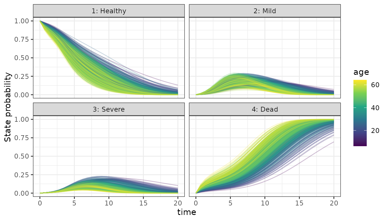

# By sex
df_bysex <- df |>
  group_by(State, time, sex) |>
  summarise(p_mean = mean(mean(prob)), .groups = "drop")
plt_sex <- ggplot(df_bysex, aes(x = time, y = p_mean, group = sex, color = sex)) +
  facet_wrap(. ~ State) +
  geom_line() +
  ylab("Mean state probability")
plt_sex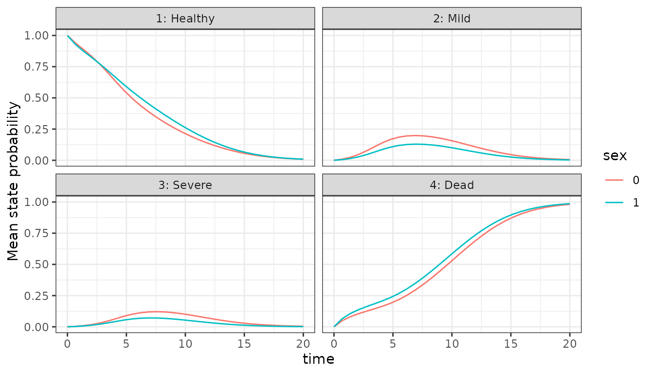

# By donor age
plt_dage <- ggplot(df, aes(x = time, y = mean(prob), group = subject_id, color = dage)) +
  facet_wrap(. ~ State) +
  geom_line(alpha = 0.25) +
  scale_color_viridis_c() +
  ylab("State probability")
plt_dage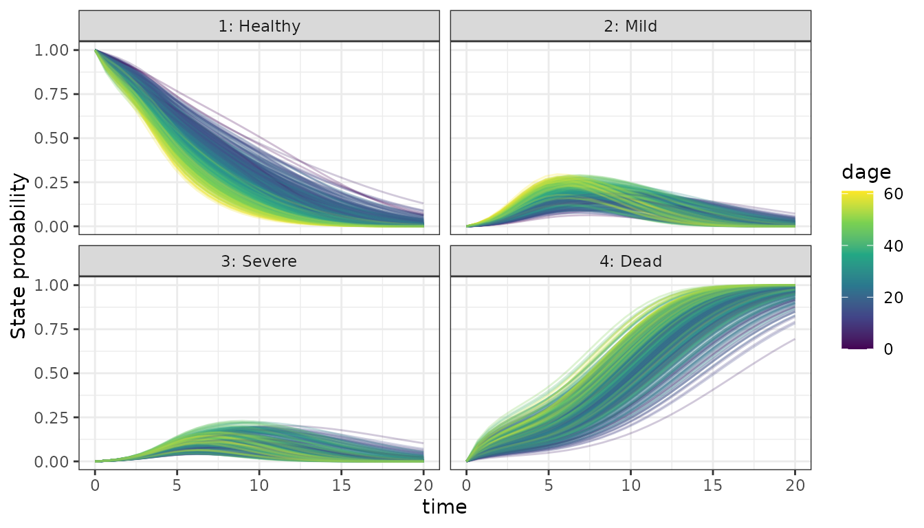

Predicting for a new subject

Here is a function for creating test data for a new subject with given covariates and given state at time 0.

create_test_subject <- function(state, dages = c(20, 30, 40, 50, 60, 70, 80), age = 60, sex = 0) {
  pdf <- NULL
  sdf <- NULL
  ldf <- NULL
  j <- 0
  for (dage in dages) {
    j <- j + 1
    sid <- paste0("test-", dage)
    pdf_j <- data.frame(path_id = j, state = state, time = c(0, 20), trans_idx = c(0, 1))
    sdf_j <- data.frame(subject_id = sid, age = age, dage = dage, sex = sex)
    ldf_j <- data.frame(path_id = j, draw_idx = 1, rep_idx = 1, subject_id = sid)
    pdf <- rbind(pdf, pdf_j)
    ldf <- rbind(ldf, ldf_j)
    sdf <- rbind(sdf, sdf_j)
  }

  pd <- PathData$new(sdf, pdf, ldf, fit$model$system$tm(), c("age", "dage", "sex"))
  JointData$new(paths = pd, dosing = NULL)
}

We can use it like this to predict the state occupancy probabilities for the same 60 years old subject with sex 0, considering what if they got the transplant from a donor of given age.

Starting healthy

dat_test <- create_test_subject(state = 1)
df_test <- p_state_df(fit, data = dat_test, oos = TRUE)
#> calling solve_trans_prob_matrix 7 x 1 times
ggplot(df_test, aes(x = time, y = mean(prob), group = subject_id, color = dage)) +
  facet_wrap(. ~ State) +
  geom_line() +
  scale_color_viridis_c() +
  ylab("State probability")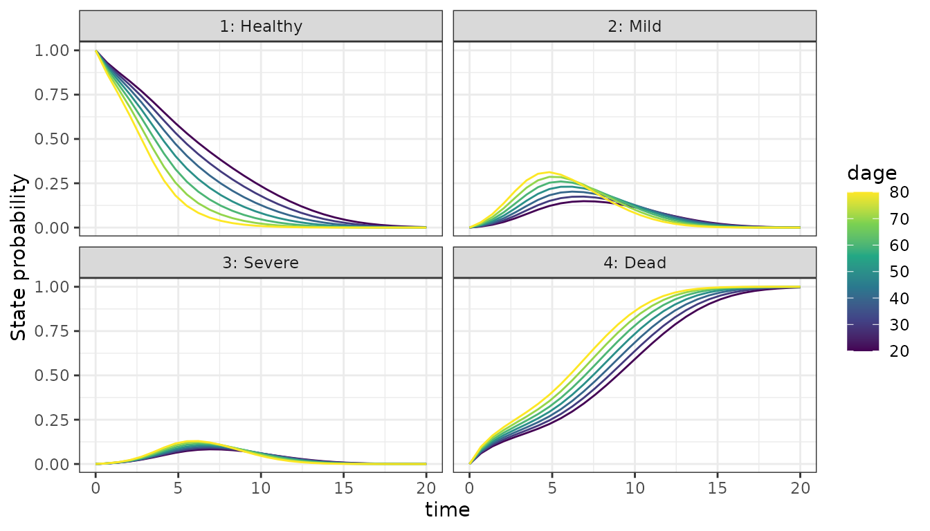

Starting from Mild CAV

dat_test <- create_test_subject(state = 2)
df_test <- p_state_df(fit, data = dat_test, oos = TRUE)
#> calling solve_trans_prob_matrix 7 x 1 times
ggplot(df_test, aes(x = time, y = mean(prob), group = subject_id, color = dage)) +
  facet_wrap(. ~ State) +
  geom_line() +
  scale_color_viridis_c() +
  ylab("State probability")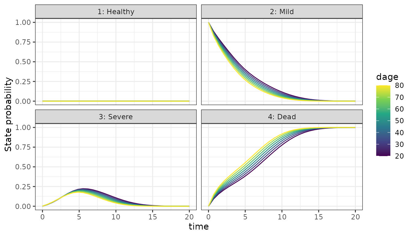

Starting from Severe CAV

dat_test <- create_test_subject(state = 3)
df_test <- p_state_df(fit, data = dat_test, oos = TRUE)
#> calling solve_trans_prob_matrix 7 x 1 times
ggplot(df_test, aes(x = time, y = mean(prob), group = subject_id, color = dage)) +
  facet_wrap(. ~ State) +
  geom_line() +
  scale_color_viridis_c() +
  ylab("State probability")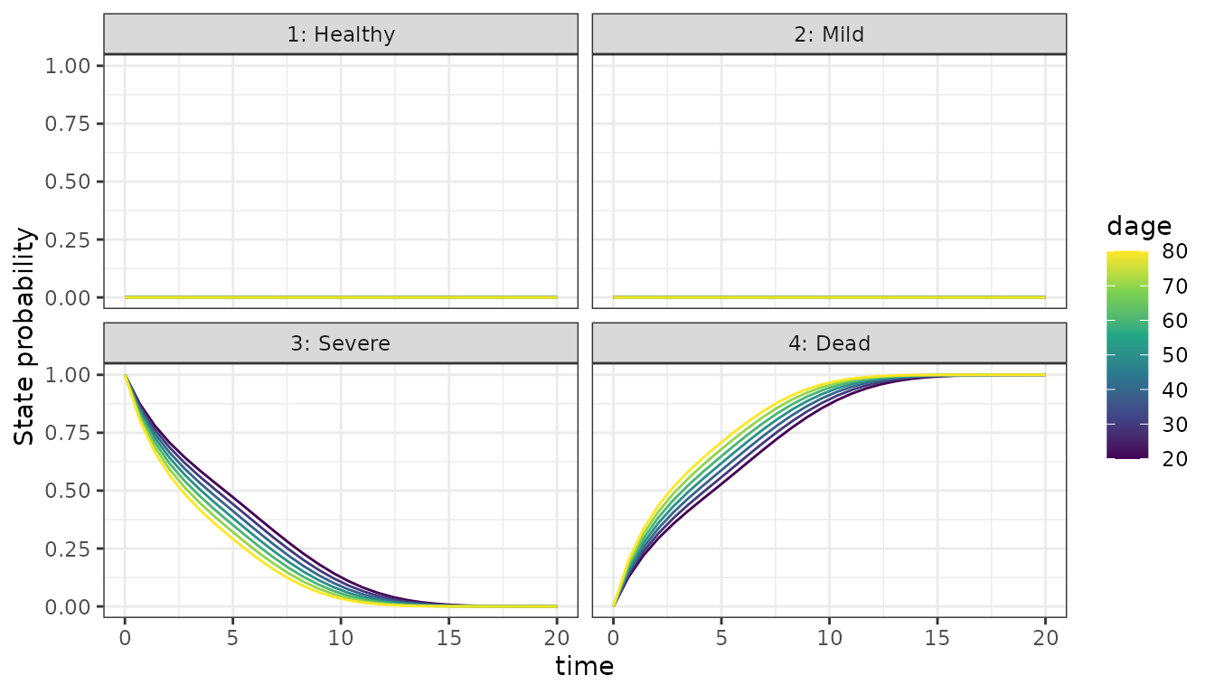

Generating paths

We simulate state paths for a single subject using the fit.

dat_test <- pd$filter(pd$subject_df$subject_id[1])
pg <- generate_paths(fit, oos = TRUE, data = dat_test, n_rep = 1000)
#> Computing hazard multipliers and getting state vector at t_start
#> Generating paths
#> Generating 1000 paths

We compute the 20-year state visit probabilities.

p1 <- p_state_visit_per_subject(pg, "Mild")
p2 <- p_state_visit_per_subject(pg, "Severe")
p3 <- p_state_visit_per_subject(pg, "Dead")
psv <- rbind(p1, p2, p3) |> left_join(pg$subject_df, by = "subject_id")
psv
#>   subject_id  prob      age dage sex
#> 1     100002 0.519 52.49589   21   0
#> 2     100002 0.265 52.49589   21   0
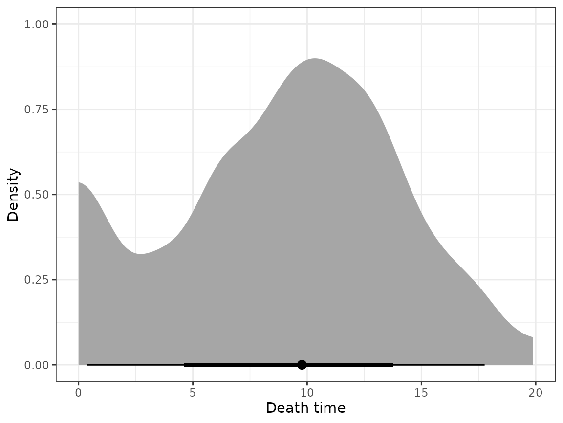
#> 3     100002 0.990 52.49589   21   0

We can study the death event time distribution for this subject.

td <- pg$as_transitions() |> filter(trans_idx > 0 & to == 4)
ggplot(td, aes(x = time)) +
  stat_halfeye() +
  xlab("Death time") +
  ylab("Density")

Juho Timonen

4th Nov 2025