Exposure-hazard multistate modeling with bmstate
Juho Timonen
20th Nov 2025
exposure-hazard.RmdThis vignette is work in progress.
Data simulation
Setup
library(bmstate)
#> Attached bmstate 0.3.3. Type ?bmstate to get started.
library(dplyr)
#>
#> Attaching package: 'dplyr'
#> The following objects are masked from 'package:stats':
#>
#>     filter, lag
#> The following objects are masked from 'package:base':
#>
#>     intersect, setdiff, setequal, union
library(tidyr)
library(tibble)
library(ggplot2)True data-generating model
# True beta
create_true_covariate_effects <- function(mod) {
  NTT <- mod$system$num_states() - 1
  C <- length(mod$covs())
  bh_true <- matrix(0, NTT, C)
  bh_true[1, 2] <- 1
  bh_true[2, 2] <- -1
  bh_true[3, 1] <- 0.3
  sn <- event_state_names(mod)
  rownames(bh_true) <- paste0("Effect on ", sn)
  colnames(bh_true) <- mod$covs()
  df <- data.frame(bh_true) |>
    rownames_to_column("event") |>
    pivot_longer(cols = -event, names_to = "covariate", values_to = "beta")
  beta_pk <- list(CL = c(0.3, -0.3), V2 = c(0.3))
  list(df = df, matrix = bh_true, pk = beta_pk)
}

# True baseline hazard parameters
create_true_baseline_hazard <- function(mod) {
  tm <- mod$system$tm()

  # Spline weights
  w_true <- matrix(0, 7, 9)
  for (j in 1:7) {
    ww <- rep(0, 9)
    if (tm$trans_df()$trans_type[j] == 2) {
      ww <- rep(-1, 9)
      ww[3:5] <- 1
    }
    if (tm$trans_df()$trans_type[j] == 3) {
      ww <- rep(-1, 9)
      ww[4:8] <- 1
    }
    w_true[j, ] <- ww
  }

  # Intercept
  w0_true <- 0.5 * 1e-3
  w0_true_vec <- rep(w0_true, 7)
  w0_true_vec[3] <- 0.1 * w0_true
  w0_true_vec[5] <- 5 * w0_true
  w0_true_vec[7] <- 20 * w0_true

  # Return
  list(w0 = w0_true_vec, w = w_true)
}

# True data-generating model
create_true_model <- function() {
  # Create models
  sn <- c("Healthy", "Bleed", "Stroke", "Dead")
  tm <- transmat_diamond(state_names = sn)
  t3yr <- 3 * 365.25
  haz_covs <- c("age")
  pk_covs <- list(
    CL = c("CrCL", "age"), V2 = "weight"
  )
  create_msm(
    tm,
    hazard_covs = haz_covs, pk_covs = pk_covs, num_knots = 8, t_max = t3yr
  )
}

# Create oracle fit draws
create_oracle_fit <- function(similar_fit, beta_true, h0_true) {
  checkmate::assert_true(similar_fit$is_point_estimate())
  weights <- similar_fit$get_draws("weights")
  weights[1, , ] <- h0_true$w
  log_w0 <- similar_fit$get_draws("log_w0")
  log_w0[1, ] <- log(h0_true$w0)

  beta_oth <- similar_fit$get_draws("beta_oth")
  beta_oth[1, , ] <- t(beta_true$matrix[, 1])
  beta_oth <- posterior::rvar(beta_oth)

  beta_xpsr <- similar_fit$get_draws("beta_xpsr")
  beta_xpsr[1, , ] <- t(beta_true$matrix[, 2])

  lp <- similar_fit$get_draws("lp__")
  lp[] <- NA
  log_z_pk <- similar_fit$get_draws("log_z_pk")
  log_z_pk[, , ] <- 0
  log_sig_pk <- similar_fit$get_draws("log_sig_pk")
  log_sig_pk[, ] <- 0
  log_mu_pk <- similar_fit$get_draws("log_mu_pk")
  log_mu_pk[, ] <- 0
  sigma_pk <- similar_fit$get_draws("sigma_pk")
  sigma_pk[] <- 0.3
  beta_CL <- similar_fit$get_draws("beta_CL")
  beta_CL[1, ] <- beta_true$pk$CL
  beta_V2 <- similar_fit$get_draws("beta_V2")
  beta_V2[1, ] <- beta_true$pk$V2

  # Create fit
  draws <- list(
    beta_oth = beta_oth,
    beta_xpsr = beta_xpsr,
    beta_CL = beta_CL,
    beta_V2 = beta_V2,
    weights = weights,
    log_z_pk = log_z_pk,
    log_sig_pk = log_sig_pk,
    log_mu_pk = log_mu_pk,
    sigma_pk = sigma_pk,
    log_w0 = log_w0,
    lp__ = lp
  )
  sd <- similar_fit$get_data()
  mod <- similar_fit$model
  MultistateModelFit$new(similar_fit$data, sd, mod, draws,
    info = "Oracle fit"
  )
}
Data simulation
mod_true <- create_true_model()
beta_true <- create_true_covariate_effects(mod_true)
h0_true <- create_true_baseline_hazard(mod_true)
simdat <- mod_true$simulate_data(
  params$N_subject,
  beta_haz = beta_true$matrix,
  beta_pk = beta_true$pk,
  w0 = h0_true$w0,
  w = h0_true$w
)
#> Recompiling Stan model
#> Using stan file at /home/runner/work/_temp/Library/bmstate/stan/msm.stan
#> Generating 600 paths
covs_dh <- unique(c(mod_true$data_covs(), "dose_amt"))
simdat_dh <- simdat$paths$subset_covariates(covs_dh, renamed_old = "dose", renamed_new = "dose_amt")
simdat_death <- as_single_event(simdat_dh, "Dead", null_state = "Healthy")

sa <- simdat$paths$subject_df$xpsr
mod_true$set_xpsr_normalizers(loc = mean(sa), scale = stats::sd(sa))
#> setting xpsr normalizers to loc = 5.34993, scale = 0.69161

simdat <- mod_true$simulate_data(
  params$N_subject,
  beta_haz = beta_true$matrix,
  beta_pk = beta_true$pk,
  w0 = h0_true$w0,
  w = h0_true$w
)
#> Generating 600 paths
print(simdat)
#> A JointData object:
#> PathData object with 600 paths
#>  * States = {Healthy, Bleed, Stroke, Dead}
#>  * Covariates = {age, CrCL, weight, dose, t_pre, t_post, conc_pre, conc_post, xpsr, ka, CL, V2, pk_lloq}
#>
#> A DosingData object with 600 subjects
Modeling
Defining models
NK <- 4
tm <- mod_true$system$tm()
pk_covs <- list(
  ka = mod_true$pk_model$ka_covs(),
  CL = mod_true$pk_model$CL_covs(),
  V2 = mod_true$pk_model$V2_covs()
)

# Exposure-hazard multistate model
mod_ms_eh <- create_msm(
  tm,
  hazard_covs = setdiff(mod_true$covs(), "xpsr"),
  pk_covs = pk_covs,
  num_knots = NK, t_max = mod_true$get_tmax()
)

# Dose-hazard multistate model
mod_ms_dh <- create_msm(
  tm,
  hazard_covs = covs_dh, num_knots = NK, t_max = mod_true$get_tmax()
)

# Survival model
tm0 <- transmat_survival(tm$states[c(1, 4)])
mod_death <- create_msm(
  tm0,
  hazard_covs = covs_dh, num_knots = NK, t_max = mod_true$get_tmax()
)
# Inference model knots
t3yr <- mod_true$get_tmax()
tt1 <- simdat$paths$transition_times()
tt2 <- simdat_dh$transition_times()
tt3 <- simdat_death$transition_times()
mod_ms_eh$set_knots(t3yr, tt1, NK)
mod_ms_dh$set_knots(t3yr, tt2, NK)
mod_death$set_knots(t3yr, tt3, NK)
# Oracle fit
fit_prelim <- fit_stan(mod_true, simdat, method = "optimize", init = 0, iter = 100)
#> Shortest time interval (0.100000000000023) is smaller than delta_grid (1.09575). Consider increasing n_grid or decreasing t_max of the model.
#> Using stan file at /home/runner/work/_temp/Library/bmstate/stan/msm.stan
#> setting xpsr normalizers to loc = 5.42315, scale = 0.56671
#> setting max conc = 9565.56038
#> Initial log joint probability = -899042
#> Iter log prob ||dx|| ||grad|| alpha alpha0 # evals Notes
#> 99 -9793.73 0.045901 1148.39 0.8822 0.8822 120
#> Iter log prob ||dx|| ||grad|| alpha alpha0 # evals Notes
#> 100 -9788.14 0.016727 786.414 1 1 121
#> Optimization terminated normally:
#> Maximum number of iterations hit, may not be at an optima
#> Finished in 0.8 seconds.
#> If these don't roughly match, consider refitting after setting xpsr normalizer loc and scale closer to estimated mean and sd. Otherwise interpret baseline hazards and xpsr effect size accodingly.
#> - xpsr normalization loc = 5.42315, mean estimated xpsr = 5.43736
#> - xpsr normalization scale = 0.56671, estimated xpsr sd = 0.70956
fit_true <- create_oracle_fit(fit_prelim, beta_true, h0_true)
fit_true$covariate_effects()
#> covariate beta target_state_idx target_state
#> 1 age 0.0 ± NA 2 Bleed
#> 2 age 0.0 ± NA 3 Stroke
#> 3 age 0.3 ± NA 4 Dead
#> 4 xpsr 1.0 ± NA 2 Bleed
#> 5 xpsr -1.0 ± NA 3 Stroke
#> 6 xpsr 0.0 ± NA 4 Dead
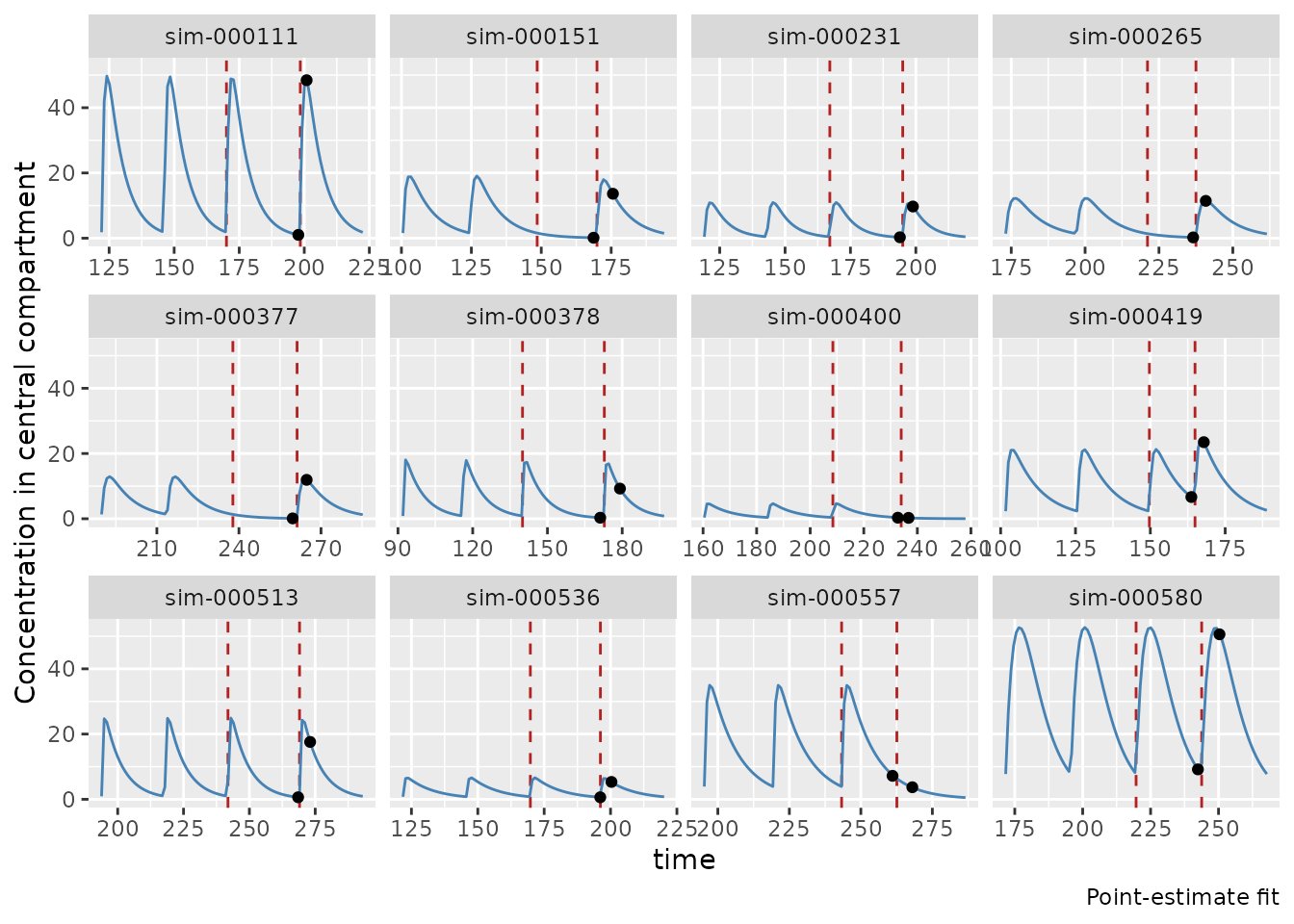
fit_true$plot_pk()
#> PK simulation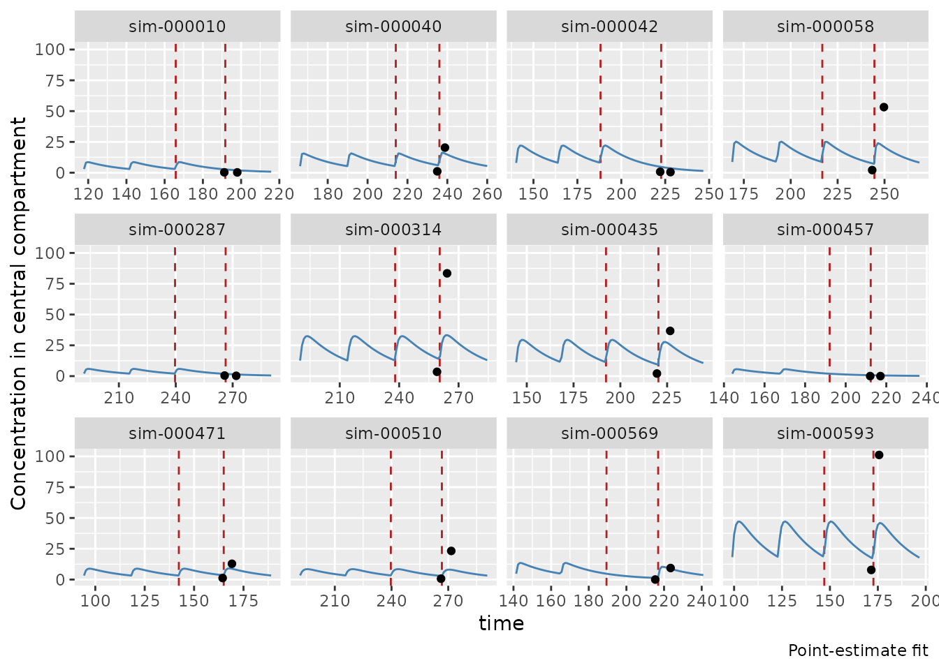
fit_true$plot_h0()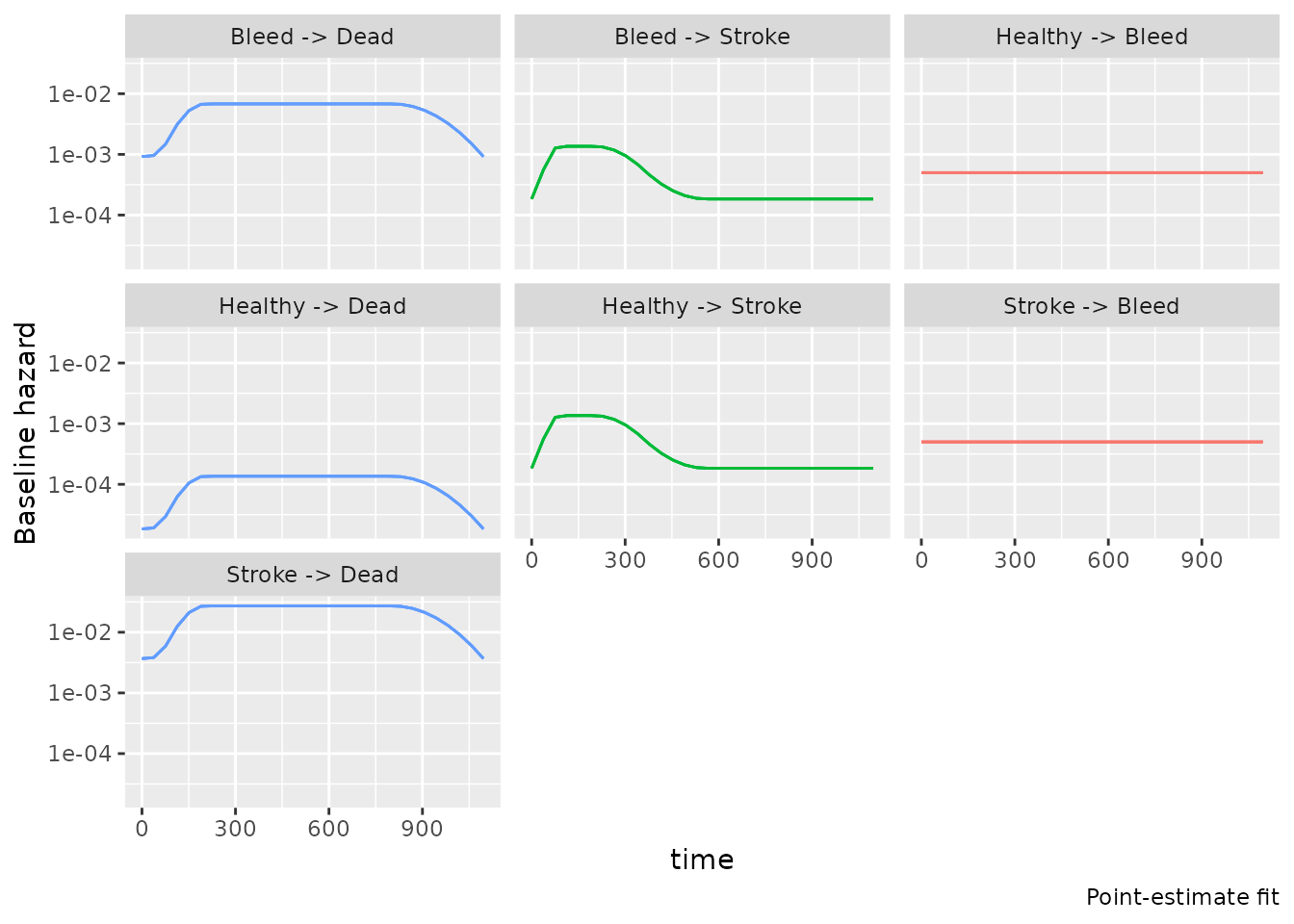
Fitting various models
fit_ms_eh <- fit_stan(mod_ms_eh, simdat, method = "optimize", init = 0)
#> Shortest time interval (0.100000000000023) is smaller than delta_grid (1.09575). Consider increasing n_grid or decreasing t_max of the model.
#> Using stan file at /home/runner/work/_temp/Library/bmstate/stan/msm.stan
#> setting xpsr normalizers to loc = 5.42315, scale = 0.56671
#> setting max conc = 9565.56038
#> Initial log joint probability = -898892
#>     Iter      log prob        ||dx||      ||grad||       alpha      alpha0  # evals  Notes
#>       99      -9603.42      0.203959       2084.08      0.5976      0.5976      119
#>     Iter      log prob        ||dx||      ||grad||       alpha      alpha0  # evals  Notes
#>      199      -8892.36     0.0260811       593.149           1           1      229
#>     Iter      log prob        ||dx||      ||grad||       alpha      alpha0  # evals  Notes
#>      299      -8465.04      0.036666       1078.48           1           1      343
#>     Iter      log prob        ||dx||      ||grad||       alpha      alpha0  # evals  Notes
#>      399       -8165.9     0.0183767       738.692           1           1      455
#>     Iter      log prob        ||dx||      ||grad||       alpha      alpha0  # evals  Notes
#>      499      -8008.91    0.00355821        746.45      0.6648      0.6648      565
#>     Iter      log prob        ||dx||      ||grad||       alpha      alpha0  # evals  Notes
#>      599      -7882.82    0.00308223       1094.79           1           1      669
#>     Iter      log prob        ||dx||      ||grad||       alpha      alpha0  # evals  Notes
#>      699      -7788.76    0.00210207        1873.5       0.621       0.621      783
#>     Iter      log prob        ||dx||      ||grad||       alpha      alpha0  # evals  Notes
#>      799      -7736.08     0.0359836       755.961           1           1      897
#>     Iter      log prob        ||dx||      ||grad||       alpha      alpha0  # evals  Notes
#>      899      -7660.32     0.0285034       808.329           1           1     1007
#>     Iter      log prob        ||dx||      ||grad||       alpha      alpha0  # evals  Notes
#>      999      -7537.49     0.0111011       1177.28           1           1     1119
#>     Iter      log prob        ||dx||      ||grad||       alpha      alpha0  # evals  Notes
#>     1099       -7482.9     0.0259127       1653.56           1           1     1230
#>     Iter      log prob        ||dx||      ||grad||       alpha      alpha0  # evals  Notes
#>     1199      -7425.37     0.0235646       3312.85      0.2649           1     1344
#>     Iter      log prob        ||dx||      ||grad||       alpha      alpha0  # evals  Notes
#>     1299      -7395.09    0.00192234       679.179           1           1     1453
#>     Iter      log prob        ||dx||      ||grad||       alpha      alpha0  # evals  Notes
#>     1399      -7375.47    0.00329343       673.567           1           1     1569
#>     Iter      log prob        ||dx||      ||grad||       alpha      alpha0  # evals  Notes
#>     1499      -7354.32    0.00937889       609.642           1           1     1678
#>     Iter      log prob        ||dx||      ||grad||       alpha      alpha0  # evals  Notes
#>     1599      -7323.88     0.0372511       1122.04           1           1     1788
#>     Iter      log prob        ||dx||      ||grad||       alpha      alpha0  # evals  Notes
#>     1699      -7262.78    0.00805707       1217.84           1           1     1900
#>     Iter      log prob        ||dx||      ||grad||       alpha      alpha0  # evals  Notes
#>     1799      -7209.87    0.00826959       1215.84           1           1     2009
#>     Iter      log prob        ||dx||      ||grad||       alpha      alpha0  # evals  Notes
#>     1899      -7181.51   0.000383597        406.75           1           1     2116
#>     Iter      log prob        ||dx||      ||grad||       alpha      alpha0  # evals  Notes
#>     1999       -7172.3     0.0058379       454.649           1           1     2225
#>     Iter      log prob        ||dx||      ||grad||       alpha      alpha0  # evals  Notes
#>     2000      -7172.23    0.00310466       394.594           1           1     2226
#> Optimization terminated normally:
#>   Maximum number of iterations hit, may not be at an optima
#> Finished in  11.2 seconds.
#> If these don't roughly match, consider refitting after setting xpsr normalizer loc and scale closer to estimated mean and sd. Otherwise interpret baseline hazards and xpsr effect size accodingly.
#>  - xpsr normalization loc = 5.42315, mean estimated xpsr = 5.51054
#>  - xpsr normalization scale = 0.56671, estimated xpsr sd = 0.96017
fit_ms_dh <- fit_stan(mod_ms_dh, simdat_dh, method = "optimize", init = 0)
#> Shortest time interval (0.100000000000001) is smaller than delta_grid (1.09575). Consider increasing n_grid or decreasing t_max of the model.
#> Using stan file at /home/runner/work/_temp/Library/bmstate/stan/msm.stan
#> Initial log joint probability = -804054
#>     Iter      log prob        ||dx||      ||grad||       alpha      alpha0  # evals  Notes
#>       99      -6390.86      0.342268       271.848           1           1      120
#>     Iter      log prob        ||dx||      ||grad||       alpha      alpha0  # evals  Notes
#>      199      -6212.14     0.0121632       16.9001      0.6773      0.6773      229
#>     Iter      log prob        ||dx||      ||grad||       alpha      alpha0  # evals  Notes
#>      299      -6205.79     0.0172344       10.0839           1           1      340
#>     Iter      log prob        ||dx||      ||grad||       alpha      alpha0  # evals  Notes
#>      399      -6202.51     0.0100091       5.67042           1           1      449
#>     Iter      log prob        ||dx||      ||grad||       alpha      alpha0  # evals  Notes
#>      499      -6198.78     0.0317216       15.1583           1           1      553
#>     Iter      log prob        ||dx||      ||grad||       alpha      alpha0  # evals  Notes
#>      599      -6196.49    0.00352212       15.3331      0.1617      0.1617      658
#>     Iter      log prob        ||dx||      ||grad||       alpha      alpha0  # evals  Notes
#>      699      -6195.72    0.00285264        2.6361           1           1      765
#>     Iter      log prob        ||dx||      ||grad||       alpha      alpha0  # evals  Notes
#>      799      -6194.37     0.0135432       13.2688           1           1      874
#>     Iter      log prob        ||dx||      ||grad||       alpha      alpha0  # evals  Notes
#>      899      -6193.72    0.00440669       3.78953           1           1      983
#>     Iter      log prob        ||dx||      ||grad||       alpha      alpha0  # evals  Notes
#>      999      -6193.61    0.00951578      0.887477           1           1     1084
#>     Iter      log prob        ||dx||      ||grad||       alpha      alpha0  # evals  Notes
#>     1099       -6192.3     0.0308932       8.71699      0.8685      0.8685     1204
#>     Iter      log prob        ||dx||      ||grad||       alpha      alpha0  # evals  Notes
#>     1199      -6190.01     0.0363073       13.3343       0.344       0.344     1313
#>     Iter      log prob        ||dx||      ||grad||       alpha      alpha0  # evals  Notes
#>     1299      -6189.68     0.0121206       3.91667      0.5025           1     1423
#>     Iter      log prob        ||dx||      ||grad||       alpha      alpha0  # evals  Notes
#>     1399      -6189.42    0.00169055       0.66537           1           1     1532
#>     Iter      log prob        ||dx||      ||grad||       alpha      alpha0  # evals  Notes
#>     1499      -6189.38      0.004892       1.28893           1           1     1637
#>     Iter      log prob        ||dx||      ||grad||       alpha      alpha0  # evals  Notes
#>     1599      -6188.91    0.00174241        2.8089      0.9912      0.9912     1746
#>     Iter      log prob        ||dx||      ||grad||       alpha      alpha0  # evals  Notes
#>     1699      -6188.79   0.000936889        1.3612       0.328           1     1860
#>     Iter      log prob        ||dx||      ||grad||       alpha      alpha0  # evals  Notes
#>     1787      -6188.78   0.000992681      0.260354      0.8284      0.8284     1953
#> Optimization terminated normally:
#>   Convergence detected: relative gradient magnitude is below tolerance
#> Finished in  5.7 seconds.
fit_death <- fit_stan(mod_death, simdat_death, method = "optimize", init = 0)
#> Using stan file at /home/runner/work/_temp/Library/bmstate/stan/msm.stan
#> Initial log joint probability = -281504
#>     Iter      log prob        ||dx||      ||grad||       alpha      alpha0  # evals  Notes
#>       99      -3522.91     0.0929614       12.8081           1           1      133
#>     Iter      log prob        ||dx||      ||grad||       alpha      alpha0  # evals  Notes
#>      175      -3522.57    0.00236701     0.0906536           1           1      224
#> Optimization terminated normally:
#>   Convergence detected: relative gradient magnitude is below tolerance
#> Finished in  0.1 seconds.
fit_ms_eh$plot_h0()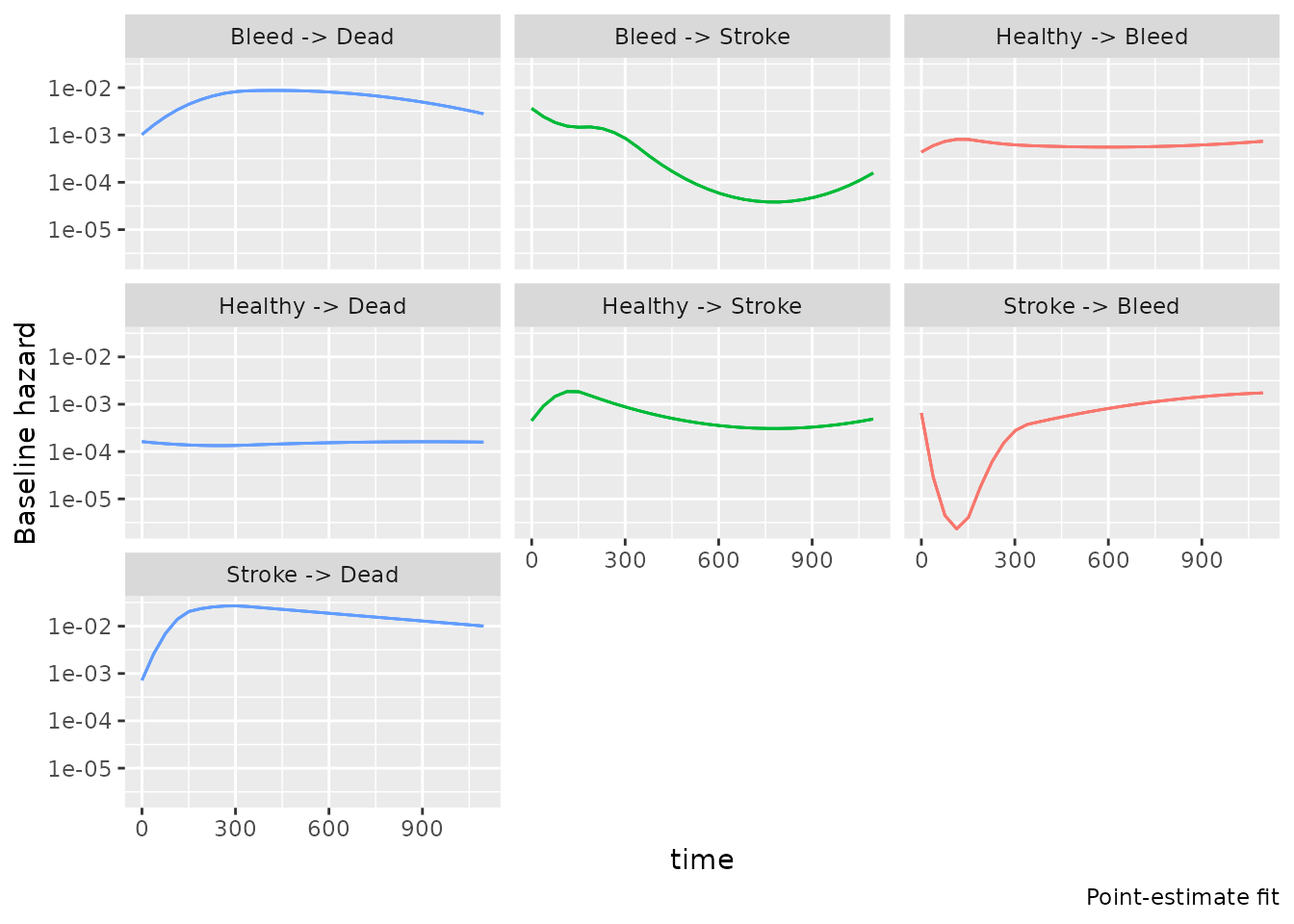
fit_ms_eh$covariate_effects()
#>   covariate        beta target_state_idx target_state
#> 1       age  0.217 ± NA                2        Bleed
#> 2       age -0.133 ± NA                3       Stroke
#> 3       age  0.222 ± NA                4         Dead
#> 4      xpsr  0.156 ± NA                2        Bleed
#> 5      xpsr -0.436 ± NA                3       Stroke
#> 6      xpsr  0.026 ± NA                4         Dead
fit_ms_dh$covariate_effects()
#>    covariate        beta target_state_idx target_state
#> 1        age  0.707 ± NA                2        Bleed
#> 2        age -0.609 ± NA                3       Stroke
#> 3        age  0.272 ± NA                4         Dead
#> 4       CrCL -0.603 ± NA                2        Bleed
#> 5       CrCL  0.504 ± NA                3       Stroke
#> 6       CrCL  0.077 ± NA                4         Dead
#> 7     weight  0.085 ± NA                2        Bleed
#> 8     weight  0.027 ± NA                3       Stroke
#> 9     weight  0.028 ± NA                4         Dead
#> 10  dose_amt  1.026 ± NA                2        Bleed
#> 11  dose_amt -1.145 ± NA                3       Stroke
#> 12  dose_amt  0.052 ± NA                4         Dead
fit_death$covariate_effects()
#>   covariate        beta target_state_idx target_state
#> 1       age -0.104 ± NA                2         Dead
#> 2      CrCL  0.152 ± NA                2         Dead
#> 3    weight  0.042 ± NA                2         Dead
#> 4  dose_amt -0.181 ± NA                2         Dead
fit_ms_eh$plot_pk()
#> PK simulation